Subsequently, one may also ask, can you do a VLOOKUP on filtered cells?
The VLOOKUP function can help you to find and return the first matching value by default whether it is a normal range or filtered list. Sometimes, you just want to vlookup and return only the visible value if there is a filtered list.
Similarly, does VLOOKUP ignore hidden rows? As you can observe the values in the hidden rows are FALSE. So the Vlookup search key won't match in this row. This way you can make the Vlookup Skips Hidden Rows in Google Sheets.
Also, how do I apply a formula to filtered cells only in Excel?
Re: Paste TO visible cells only in a filtered cells only
- copy the formula or value to the clipboard.
- select the filtered column.
- hit F5 or Ctrl+G to open the Go To dialog.
- Click Special.
- click "Visible cells only" and OK.
- hit Ctrl+V to paste.
How do you sum only filtered visible cells in Excel with criteria?
Just organize your data in table (Ctrl + T) or filter the data the way you want by clicking the Filter button. After that, select the cell immediately below the column you want to total, and click the AutoSum button on the ribbon. A SUBTOTAL formula will be inserted, summing only the visible cells in the column.May 18, 2016
Related Question Answers
How do I do a VLOOKUP with two conditions?
VLOOKUP with Multiple Criteria – Using a Helper Column- Insert a Helper Column between column B and C.
- Use the following formula in the helper column:=A2&â€|â€&B2.
- Use the following formula in G3 =VLOOKUP($F3&â€|â€&G$2,$C$2:$D$19,2,0)
- Copy for all the cells.
How do you reference a cell in a filtered table?
Change the last sentence to read The report has been filtered to show the responses for '{filter}' ( cases). Place the cursor after the open bracket, click the [Insert] button and select Cell Values Field… from the options. The New Cell Values dialog opens. Enter the Cell Reference for the Base cell in your table.How do you get the summary of filtered data in Excel?
Using the Subtotal Function to Sum Filtered Data in Excel- Display workbook in Excel containing data to be filtered.
- Click anywhere in the data set.
- Apply filter on data.
- Click below the data to sum.
- Enter the Subtotal formula to sum the filtered data.
Can you do a VLOOKUP with hidden columns?
If you are familiar with the VLOOKUP command in Excel you may be interested to know that Vlookup counts hidden columns as well as the visible columns when deciding which columns information to bring back. the Col Index Number portion specifies which column of the highlighted table array should be pulled through.Jan 21, 2015How do you use VLOOKUP function in Excel?
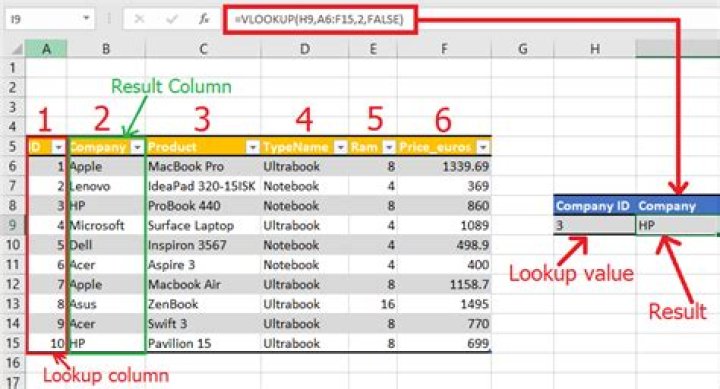
- In the Formula Bar, type =VLOOKUP().
- In the parentheses, enter your lookup value, followed by a comma.
- Enter your table array or lookup table, the range of data you want to search, and a comma: (H2,B3:F25,
- Enter column index number.
- Enter the range lookup value, either TRUE or FALSE.
What is Excel VLOOKUP?
VLOOKUP stands for 'Vertical Lookup'. It is a function that makes Excel search for a certain value in a column (the so called 'table array'), in order to return a value from a different column in the same row.How do you use the filter function in Excel?
To filter with search:- Select the Data tab, then click the Filter command. A drop-down arrow will appear in the header cell for each column.
- Click the drop-down arrow for the column you want to filter.
- The Filter menu will appear.
- When you're done, click OK.
- The worksheet will be filtered according to your search term.
How do you paste in a filtered column skipping the hidden cells?
This shortcut lets you select only the visible rows, while skipping the hidden cells. Press CTRL+C or right-click->Copy to copy these selected rows. Select the first cell where you want to paste the copied cells. Press CTRL+V or right-click->Paste to paste the cells.How do you skip hidden cells in formula?
Select a blank cell you will place the counting result into, type the formula =SUBTOTAL(102,C2:C22) (C2:C22 is the range where you want to count ignoring manually hidden cells and rows) into it, and press the Enter key.Can you use formulas on filtered data in Excel?
You can use AutoCalculate to quickly view calculations relevant to the filtered data. You also can insert simple formulas into a worksheet using the AutoSum button on the Standard toolbar. There are two ways you can find the total of a group of filtered cells.How do I paste into a filtered column?
If you want to pasting cells into a hidden or filtered cells, you need to select the visible blank cells firstly with Alt + ; shortcut, and then just press Ctrl + C keys to copy the selected cells, and then press Ctrl + V to paste your data into the selected visible cells.Aug 29, 2019How do I use Countif filtered data?
Find a blank cell and enter the formula =COUNTIFS(B2:B18,"Pear",G2:G18,"1"), and press the Enter key. (Note: In the formula of =COUNTIFS(B2:B18,"Pear",G2:G18,"1"), the B2:B18 and G2:G18 are ranges you will count, and "Pear" and "1" are criteria you will count by.) Now you will get the count number at once.How do I hide filtered data in Excel?
Right click on the column you want to hide and then click “Hide.†You can hide multiple columns this way if you have them all selected. One last look at the data set. If you want to see the hidden information again, simply right click on the space the column should be and click “Unhide.â€Jan 28, 2020How do I copy and paste only visible cells?
Copy & Paste Visible Cells- Select the entire range you want to copy.
- Press Alt+; to select the visible cells only.
- Copy the range – Press Ctrl+C or Right-click>Copy.
- Select the cell or range that you want to paste to.
- Paste the range – Press Ctrl+V or Right-click>Paste.